Modelling a Coherently Polarised Aperture

This example uses the frequency domain lyceanem.models.frequency_domain.calculate_farfield() function to predict the farfield pattern for a linearly polarised aperture. This could represent an antenna array without any beamforming weights.

import copy

import numpy as np

Setting Farfield Resolution and Wavelength

LyceanEM uses Elevation and Azimuth to record spherical coordinates, ranging from -180 to 180 degrees in azimuth, and from -90 to 90 degrees in elevation. In order to launch the aperture projection function, the resolution in both azimuth and elevation is requried. In order to ensure a fast example, 37 points have been used here for both, giving a total of 1369 farfield points.

The wavelength of interest is also an important variable for antenna array analysis, so we set it now for 10GHz, an X band aperture.

az_res = 181
elev_res = 181
wavelength = 3e8 / 10e9

Geometries

In order to make things easy to start, an example geometry has been included within LyceanEM for a UAV, and the triangle structures can be accessed by importing the data subpackage

import lyceanem.tests.reflectordata as data

body = data.UAV_Demo(wavelength * 0.5)
array = data.UAV_Demo_Aperture(wavelength * 0.5)

C:\Users\lycea\miniconda3\envs\CudaDevelopment\Lib\site-packages\meshio\stl\_stl.py:40: RuntimeWarning: overflow encountered in scalar multiply
  if 84 + num_triangles * 50 == filesize_bytes:
C:\Users\lycea\miniconda3\envs\CudaDevelopment\Lib\site-packages\meshio\stl\_stl.py:40: RuntimeWarning: overflow encountered in scalar multiply
  if 84 + num_triangles * 50 == filesize_bytes:

---

from lyceanem.base_classes import structures, points, antenna_structures

blockers = structures([body])
aperture = points([array])
array_on_platform = antenna_structures(blockers, aperture)
from lyceanem.models.frequency_domain import calculate_farfield


import pyvista as pv

Visualising the Platform and Array

pl = pv.Plotter()
pl.add_mesh(pv.from_meshio(body), color="green")
pl.add_mesh(pv.from_meshio(array))
pl.add_axes()
pl.show()

Static Scene

Interactive Scene

---

desired_E_axis = np.zeros((1, 3), dtype=np.float32)
desired_E_axis[0, 1] = 1.0

Etheta, Ephi = calculate_farfield(
    array_on_platform.export_all_points(),
    array_on_platform.export_all_structures(),
    array_on_platform.excitation_function(
        desired_e_vector=desired_E_axis, wavelength=wavelength, transmit_power=1.0
    ),
    az_range=np.linspace(-180, 180, az_res),
    el_range=np.linspace(-90, 90, elev_res),
    wavelength=wavelength,
    farfield_distance=20,
    project_vectors=False,
    beta=(2 * np.pi) / wavelength,
)

C:\Users\lycea\miniconda3\envs\CudaDevelopment\Lib\site-packages\lyceanem\electromagnetics\empropagation.py:3719: ComplexWarning: Casting complex values to real discards the imaginary part
  uvn_axes[2, :] = point_vector
C:\Users\lycea\miniconda3\envs\CudaDevelopment\Lib\site-packages\lyceanem\electromagnetics\empropagation.py:3736: ComplexWarning: Casting complex values to real discards the imaginary part
  uvn_axes[0, :] = np.cross(local_axes[2, :], point_vector) / np.linalg.norm(
C:\Users\lycea\miniconda3\envs\CudaDevelopment\Lib\site-packages\lyceanem\electromagnetics\empropagation.py:3758: ComplexWarning: Casting complex values to real discards the imaginary part
  uvn_axes[1, :] = np.cross(point_vector, uvn_axes[0, :]) / np.linalg.norm(
C:\Users\lycea\miniconda3\envs\CudaDevelopment\Lib\site-packages\cuda\core\experimental\_linker.py:189: RuntimeWarning: nvJitLink is not installed or too old (<12.3). Therefore it is not usable and the culink APIs will be used instead.
  _lazy_init()

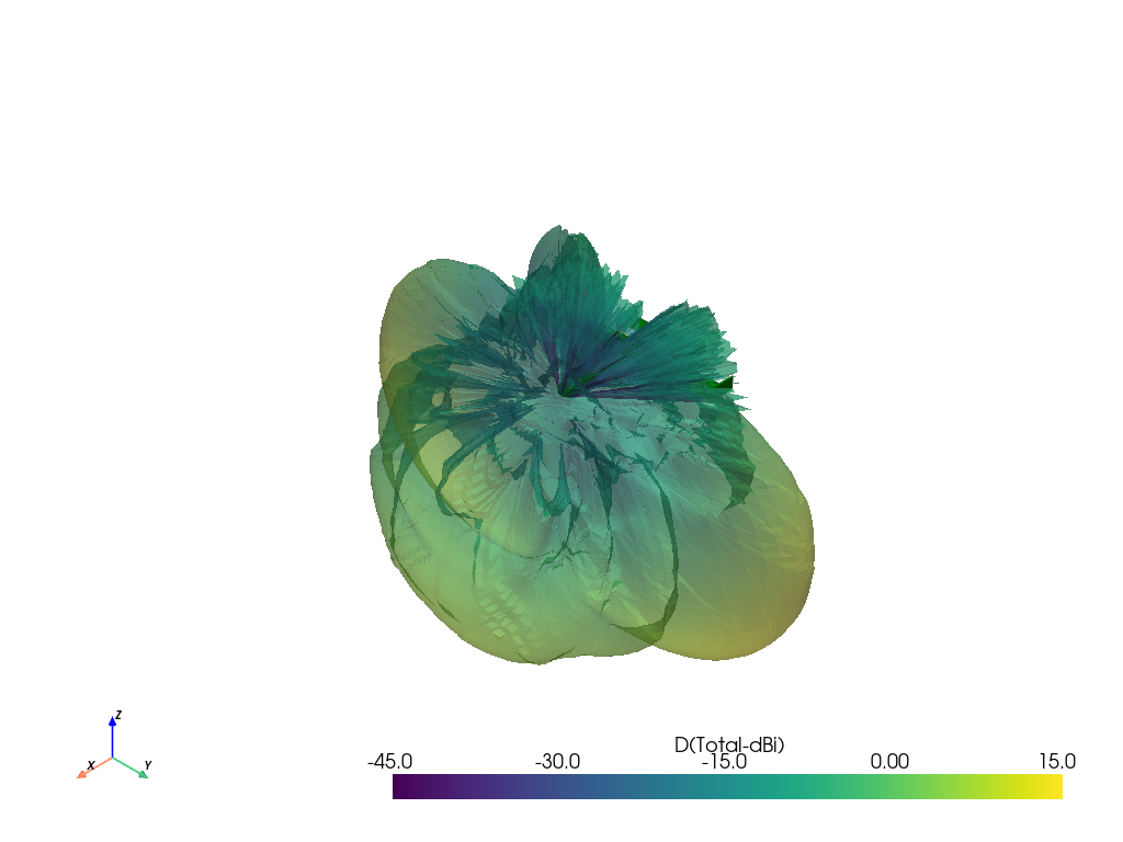
Storing and Manipulating Antenna Patterns

The resultant antenna pattern can be stored in lyceanem.base.antenna_pattern as it has been modelled as one distributed aperture, the advantage of this class is the integrated display, conversion and export functions. It is very simple to define, and save the pattern, and then display with a call to lyceanem.base.antenna_pattern.display_pattern(). This produces 3D polar plots which can be manipulated to give a better view of the whole pattern, but if contour plots are required, then this can also be produced by passing plottype=’Contour’ to the function.

from lyceanem.base_classes import antenna_pattern

UAV_Static_Pattern = antenna_pattern(
    azimuth_resolution=az_res, elevation_resolution=elev_res
)
UAV_Static_Pattern.pattern[:, :, 0] = Etheta.reshape(elev_res, az_res)
UAV_Static_Pattern.pattern[:, :, 1] = Ephi.reshape(elev_res, az_res)

UAV_Static_Pattern.display_pattern(desired_pattern="Power")

UAV_Static_Pattern.display_pattern(plottype="Contour")

pattern_mesh = UAV_Static_Pattern.pattern_mesh()

from lyceanem.electromagnetics.beamforming import create_display_mesh
from lyceanem.electromagnetics.emfunctions import Directivity
pattern_mesh=Directivity(pattern_mesh)
display_mesh = create_display_mesh(pattern_mesh, label="D(Total)", dynamic_range=60)
display_mesh.point_data["D(Total-dBi)"] = 10 * np.log10(
    display_mesh.point_data["D(Total)"]
)
display_mesh.point_data["D(Total-dBi)"][np.isinf(display_mesh.point_data["D(Total-dBi)"])]=-200
plot_max = 5 * np.ceil(np.nanmax(display_mesh.point_data["D(Total-dBi)"]) / 5)

• 
• 
• 

C:\Users\lycea\miniconda3\envs\CudaDevelopment\Lib\site-packages\lyceanem\electromagnetics\beamforming.py:1277: RuntimeWarning: divide by zero encountered in log10
  logdata = 10 * np.log10(data)
C:\Users\lycea\miniconda3\envs\CudaDevelopment\Lib\site-packages\lyceanem\electromagnetics\beamforming.py:1280: RuntimeWarning: divide by zero encountered in log10
  logdata = 20 * np.log10(data)
C:\Users\lycea\miniconda3\envs\CudaDevelopment\Lib\site-packages\lyceanem\electromagnetics\beamforming.py:1280: RuntimeWarning: divide by zero encountered in log10
  logdata = 20 * np.log10(data)
C:\Users\lycea\miniconda3\envs\CudaDevelopment\Lib\site-packages\lyceanem\electromagnetics\emfunctions.py:539: RuntimeWarning: divide by zero encountered in log10
  field_data.point_data["Poynting_Vector_(Magnitude_(dBW/m2))"] = 10 * np.log10(
C:\Users\lycea\miniconda3\envs\CudaDevelopment\Lib\site-packages\lyceanem\electromagnetics\beamforming.py:1617: RuntimeWarning: divide by zero encountered in log10
  logdata = log_multiplier * np.log10(pattern_mesh.point_data[label])
C:\Users\lycea\PycharmProjects\LyceanEM-Python\docs\source\examples\02_coherently_polarised_array.py:114: RuntimeWarning: divide by zero encountered in log10
  display_mesh.point_data["D(Total-dBi)"] = 10 * np.log10(

Visualise the Platform and the resultant Pattern

pl = pv.Plotter()
pl.add_mesh(pv.from_meshio(body), color="green")
pl.add_mesh(pv.from_meshio(array), color="aqua")
pl.add_mesh(
    display_mesh, scalars="D(Total-dBi)", clim=[plot_max - 60, plot_max],opacity=0.5
)
pl.add_axes()
pl.show()

Static Scene

Interactive Scene