Note
Go to the end to download the full example code.
Modelling Different Farfield Polarisations
This example uses the frequency domain lyceanem.models.frequency_domain.calculate_farfield() function to predict
the farfield pattern for a linearly polarised aperture. This could represent an antenna array without any beamforming
weights.
import numpy as np
Setting Farfield Resolution and Wavelength
LyceanEM uses Elevation and Azimuth to record spherical coordinates, ranging from -180 to 180 degrees in azimuth, and from -90 to 90 degrees in elevation. In order to launch the aperture projection function, the resolution in both azimuth and elevation is required. In order to ensure a fast example, 37 points have been used here for both, giving a total of 1369 farfield points.
The wavelength of interest is also an important variable for antenna array analysis, so we set it now for 10GHz, an X band aperture.
az_res = 37
elev_res = 37
wavelength = 3e8 / 10e9
Generating consistent point source to explore farfield polarisations, and rotating the source
from lyceanem.base_classes import points,structures,antenna_structures
import meshio

import lyceanem.geometry.targets as TL
import lyceanem.geometry.geometryfunctions as GF

transmit_horn_structure, transmitting_antenna_surface_coords = TL.meshedHorn(
    58e-3, 58e-3, 128e-3, 2e-3, 0.21, wavelength*0.5
)
aperture=points([transmitting_antenna_surface_coords])
blockers=structures([transmit_horn_structure])
point_antenna=antenna_structures(blockers, aperture)


from lyceanem.models.frequency_domain import calculate_farfield
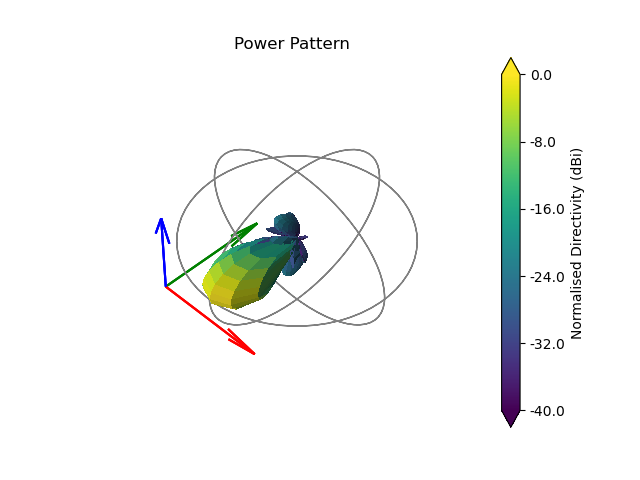
The first source polarisation is based upon the u-vector of the source point. When the excitation_function method of the antenna structure class is used, it will calculate the appropriate polarisation vectors based upon the local normal vectors.
desired_E_axis = np.zeros((1, 3), dtype=np.complex64)
desired_E_axis[0, 0] = 1.0
Etheta, Ephi = calculate_farfield(
    point_antenna.export_all_points(),
    point_antenna.export_all_structures(),
    point_antenna.excitation_function(desired_e_vector=desired_E_axis),
    az_range=np.linspace(-180, 180, az_res),
    el_range=np.linspace(-90, 90, elev_res),
    wavelength=wavelength,
    farfield_distance=20,
    elements=False,
    project_vectors=False,
    beta=(2*np.pi)/wavelength
)
C:\Users\lycea\miniconda3\envs\CudaDevelopment\Lib\site-packages\numba_cuda\numba\cuda\dispatcher.py:693: NumbaPerformanceWarning: Grid size 86 will likely result in GPU under-utilization due to low occupancy.
  warn(NumbaPerformanceWarning(msg))
C:\Users\lycea\miniconda3\envs\CudaDevelopment\Lib\site-packages\numba_cuda\numba\cuda\dispatcher.py:693: NumbaPerformanceWarning: Grid size 44 will likely result in GPU under-utilization due to low occupancy.
  warn(NumbaPerformanceWarning(msg))
Antenna Pattern class is used to manipulate and record antenna patterns
from lyceanem.base_classes import antenna_pattern

u_pattern = antenna_pattern(
    azimuth_resolution=az_res, elevation_resolution=elev_res
)
u_pattern.pattern[:, :, 0] = Etheta.reshape(elev_res,az_res)
u_pattern.pattern[:, :, 1] = Ephi.reshape(elev_res,az_res)
u_pattern.display_pattern(desired_pattern='Power')

C:\Users\lycea\miniconda3\envs\CudaDevelopment\Lib\site-packages\lyceanem\electromagnetics\beamforming.py:1277: RuntimeWarning: divide by zero encountered in log10
  logdata = 10 * np.log10(data)
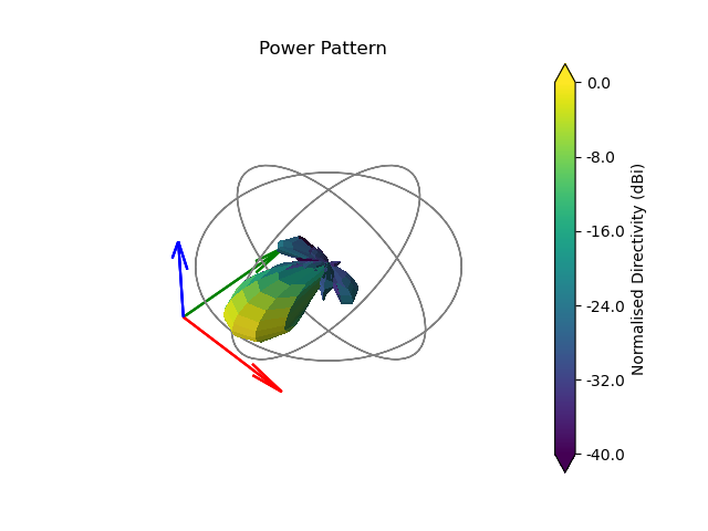
The second source polarisation is based upon the v-vector of the source point.
desired_E_axis = np.zeros((1, 3), dtype=np.complex64)
desired_E_axis[0, 1] = 1.0
Etheta, Ephi = calculate_farfield(
    point_antenna.export_all_points(),
    point_antenna.export_all_structures(),
    point_antenna.excitation_function(desired_e_vector=desired_E_axis),
    az_range=np.linspace(-180, 180, az_res),
    el_range=np.linspace(-90, 90, elev_res),
    wavelength=wavelength,
    farfield_distance=20,
    elements=False,
    project_vectors=False,
    beta=(2*np.pi)/wavelength
)


v_pattern = antenna_pattern(
    azimuth_resolution=az_res, elevation_resolution=elev_res
)
v_pattern.pattern[:, :, 0] = Etheta.reshape(elev_res,az_res)
v_pattern.pattern[:, :, 1] = Ephi.reshape(elev_res,az_res)
v_pattern.display_pattern(desired_pattern='Power')

C:\Users\lycea\miniconda3\envs\CudaDevelopment\Lib\site-packages\lyceanem\electromagnetics\beamforming.py:1277: RuntimeWarning: divide by zero encountered in log10
  logdata = 10 * np.log10(data)
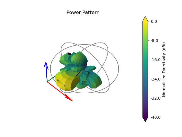
The third source polarisation is based upon the n-vector of the source point. Aligned with the source point normal.
desired_E_axis = np.zeros((1, 3), dtype=np.complex64)
desired_E_axis[0, 2] = 1.0
Etheta, Ephi = calculate_farfield(
    point_antenna.export_all_points(),
    point_antenna.export_all_structures(),
    point_antenna.excitation_function(desired_e_vector=desired_E_axis),
    az_range=np.linspace(-180, 180, az_res),
    el_range=np.linspace(-90, 90, elev_res),
    wavelength=wavelength,
    farfield_distance=20,
    elements=False,
    project_vectors=False,
    beta=(2*np.pi)/wavelength
)

n_pattern = antenna_pattern(
    azimuth_resolution=az_res, elevation_resolution=elev_res
)
n_pattern.pattern[:, :, 0] = Etheta.reshape(elev_res,az_res)
n_pattern.pattern[:, :, 1] = Ephi.reshape(elev_res,az_res)
n_pattern.display_pattern(desired_pattern='Power')

C:\Users\lycea\miniconda3\envs\CudaDevelopment\Lib\site-packages\lyceanem\electromagnetics\beamforming.py:1277: RuntimeWarning: divide by zero encountered in log10
  logdata = 10 * np.log10(data)
The point source can then be rotated, by providing a rotation matrix, and the u,v,n directions are moved with it in a consistent way.
from scipy.spatial.transform import Rotation as R

r=R.from_euler('xyz', np.radians(np.asarray([90.0,0.0,0.0])))
point_antenna.rotate_antenna(r.as_matrix())

desired_E_axis = np.zeros((1, 3), dtype=np.complex64)
desired_E_axis[0, 0] = 1.0
Etheta, Ephi = calculate_farfield(
    point_antenna.export_all_points(),
    point_antenna.export_all_structures(),
    point_antenna.excitation_function(desired_e_vector=desired_E_axis),
    az_range=np.linspace(-180, 180, az_res),
    el_range=np.linspace(-90, 90, elev_res),
    wavelength=wavelength,
    farfield_distance=20,
    elements=False,
    project_vectors=False,
    beta=(2*np.pi)/wavelength
)
u_pattern.pattern[:, :, 0] = Etheta.reshape(elev_res,az_res)
u_pattern.pattern[:, :, 1] = Ephi.reshape(elev_res,az_res)
u_pattern.display_pattern(desired_pattern='Power')


desired_E_axis = np.zeros((1, 3), dtype=np.complex64)
desired_E_axis[0, 1] = 1.0
Etheta, Ephi = calculate_farfield(
    point_antenna.export_all_points(),
    point_antenna.export_all_structures(),
    point_antenna.excitation_function(desired_e_vector=desired_E_axis),
    az_range=np.linspace(-180, 180, az_res),
    el_range=np.linspace(-90, 90, elev_res),
    wavelength=wavelength,
    farfield_distance=20,
    elements=False,
    project_vectors=False,
    beta=(2*np.pi)/wavelength
)
v_pattern.pattern[:, :, 0] = Etheta.reshape(elev_res,az_res)
v_pattern.pattern[:, :, 1] = Ephi.reshape(elev_res,az_res)
v_pattern.display_pattern(desired_pattern='Power')


desired_E_axis = np.zeros((1, 3), dtype=np.complex64)
desired_E_axis[0, 2] = 1.0
Etheta, Ephi = calculate_farfield(
    point_antenna.export_all_points(),
    point_antenna.export_all_structures(),
    point_antenna.excitation_function(desired_e_vector=desired_E_axis),
    az_range=np.linspace(-180, 180, az_res),
    el_range=np.linspace(-90, 90, elev_res),
    wavelength=wavelength,
    farfield_distance=20,
    elements=False,
    project_vectors=False,
    beta=(2*np.pi)/wavelength
)
n_pattern.pattern[:, :, 0] = Etheta.reshape(elev_res,az_res)
n_pattern.pattern[:, :, 1] = Ephi.reshape(elev_res,az_res)
n_pattern.display_pattern(desired_pattern='Power')
C:\Users\lycea\miniconda3\envs\CudaDevelopment\Lib\site-packages\numba_cuda\numba\cuda\dispatcher.py:693: NumbaPerformanceWarning: Grid size 49 will likely result in GPU under-utilization due to low occupancy.
  warn(NumbaPerformanceWarning(msg))
C:\Users\lycea\miniconda3\envs\CudaDevelopment\Lib\site-packages\lyceanem\electromagnetics\beamforming.py:1277: RuntimeWarning: divide by zero encountered in log10
  logdata = 10 * np.log10(data)
C:\Users\lycea\miniconda3\envs\CudaDevelopment\Lib\site-packages\lyceanem\electromagnetics\beamforming.py:1277: RuntimeWarning: divide by zero encountered in log10
  logdata = 10 * np.log10(data)
C:\Users\lycea\miniconda3\envs\CudaDevelopment\Lib\site-packages\lyceanem\electromagnetics\beamforming.py:1277: RuntimeWarning: divide by zero encountered in log10
  logdata = 10 * np.log10(data)
Total running time of the script: (0 minutes 1.993 seconds)