Array Beamforming

This example uses the frequency domain lyceanem.models.frequency_domain.calculate_farfield() function to predict the farfield patterns for a linearly polarised aperture with multiple elements. This is then beamformed to all farfield points using multiple open loop beamforming algorithms to attemp to ‘map’ out the acheivable beamforming for the antenna array using lyceanem.electromagnetics.beamforming.MaximumDirectivityMap().

The Steering Efficiency can then be evaluated using lyceanem.electromagnetics.beamforming.Steering_Efficiency() for the resultant achieved beamforming.

import numpy as np

Setting Farfield Resolution and Wavelength

LyceanEM uses Elevation and Azimuth to record spherical coordinates, ranging from -180 to 180 degrees in azimuth, and from -90 to 90 degrees in elevation. In order to launch the aperture projection function, the resolution in both azimuth and elevation is requried. In order to ensure a fast example, 37 points have been used here for both, giving a total of 1369 farfield points.

The wavelength of interest is also an important variable for antenna array analysis, so we set it now for 10GHz, an X band aperture.

az_res = 181
elev_res = 37
wavelength = 3e8 / 10e9

Geometries

In order to make things easy to start, an example geometry has been included within LyceanEM for a UAV, and the mesh structures can be accessed by importing the data subpackage

import lyceanem.tests.reflectordata as data

body, array, source_coords = data.exampleUAV(10e9)

from lyceanem.base_classes import structures

blockers = structures([body, array])

Model Farfield Array Patterns

The same function is used to predict the farfield pattern of each element in the array, but the variable ‘elements’ is set as True, instructing the function to return the antenna patterns as 3D arrays arranged with axes element, elevation points, and azimuth points. These can then be beamformed using the desired beamforming algorithm. LyceanEM currently includes two open loop algorithms for phase weights lyceanem.electromagnetics.beamforming.EGCWeights(), and lyceanem.electromagnetics.beamforming.WavefrontWeights()

from lyceanem.models.frequency_domain import calculate_farfield

desired_E_axis = np.zeros((1, 3), dtype=np.float32)
desired_E_axis[0, 1] = 1.0

Etheta, Ephi = calculate_farfield(
    source_coords,
    blockers,
    desired_E_axis,
    az_range=np.linspace(-180, 180, az_res),
    el_range=np.linspace(-90, 90, elev_res),
    wavelength=wavelength,
    farfield_distance=20,
    elements=True,
    project_vectors=True,
    beta=(2*np.pi)/wavelength
)


from lyceanem.electromagnetics.beamforming import MaximumDirectivityMap

az_range = np.linspace(-180, 180, az_res)
el_range = np.linspace(-90, 90, elev_res)
directivity_map = MaximumDirectivityMap(
    Etheta, Ephi, source_coords, wavelength, az_range, el_range
)

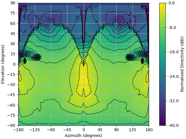
from lyceanem.electromagnetics.beamforming import PatternPlot

az_mesh, elev_mesh = np.meshgrid(az_range, el_range)

PatternPlot(
    directivity_map[:, :, 2], az_mesh, elev_mesh, logtype="power", plottype="Contour"
)

from lyceanem.electromagnetics.beamforming import Steering_Efficiency

setheta, sephi, setot = Steering_Efficiency(
    directivity_map[:, :, 0],
    directivity_map[:, :, 1],
    directivity_map[:, :, 2],
    np.radians(np.diff(el_range)[0]),
    np.radians(np.diff(az_range)[0]),
    4 * np.pi,
)

print("Steering Effciency of {:3.1f}%".format(setot))


print(
    "Maximum Directivity of {:3.1f} dBi".format(
        np.max(10 * np.log10(directivity_map[:, :, 2]))
    )
)