Note
Go to the end to download the full example code.
Antenna Array Validation
This example uses some custom functions to import antenna array measurements from a 32 element antenna array panel, and simulate the same antenna array within LyceanEM. Some basic functions are included to import the hdf5 file, and demostrate a suitable method for generating an equivalent model antenna array using gmsh.
The measurement file can be found at https://osf.io/64yaj/files/osfstorage/6867f249514c2235de49f20e , and should be placed in the same folder as this script.
import pyvista as pv
import meshio
import numpy as np
from scipy.constants import speed_of_light


def Beamform(Antennas, weights):
    """
    Assuming all the sample fields in the Antennas list are the same points with only the element differing, the weights array will be used to calculate a resultant array pattern,

    """
    field_shape = Antennas[0].point_data["Ex-Real"].shape
    beamformed_map = np.zeros((field_shape[0], 3), dtype=np.complex64)

    for element in range(len(Antennas)):
        beamformed_map[:, 0] += (
            (
                Antennas[element].point_data["Ex-Real"]
                + 1j * Antennas[element].point_data["Ex-Imag"]
            )
            * weights[element].reshape(1, -1)
        ).ravel()
        beamformed_map[:, 1] += (
            (
                Antennas[element].point_data["Ey-Real"]
                + 1j * Antennas[element].point_data["Ey-Imag"]
            )
            * weights[element].reshape(1, -1)
        ).ravel()
        beamformed_map[:, 2] += (
            (
                Antennas[element].point_data["Ez-Real"]
                + 1j * Antennas[element].point_data["Ez-Imag"]
            )
            * weights[element].reshape(1, -1)
        ).ravel()

    beamformed_pattern = meshio.Mesh(
        points=Antennas[0].points,
        cells=[("triangle", Antennas[0].cells[0].data)],
        point_data={
            "Normals": Antennas[0].point_data["Normals"],
            "Ex-Real": np.real(beamformed_map[:, 0]),
            "Ex-Imag": np.imag(beamformed_map[:, 0]),
            "Ey-Real": np.real(beamformed_map[:, 1]),
            "Ey-Imag": np.imag(beamformed_map[:, 1]),
            "Ez-Real": np.real(beamformed_map[:, 2]),
            "Ez-Imag": np.imag(beamformed_map[:, 2]),
        },
    )

    return beamformed_pattern


def Panel_Array_data():
    from pathlib import Path
    from lyceanem.geometry.geometryfunctions import compute_areas, compute_normals
    from lyceanem.electromagnetics.emfunctions import update_electric_fields

    dataset_location = Path("Panel_Array_Measurements.hdf5")
    import h5py

    with h5py.File(dataset_location, "r") as f1:
        # print(f1.name)
        # print(f1['Fields'].keys())
        antennas = []
        for field_inc in range(f1["Metadata"]["Element Positions"][:].shape[0]):
            pattern_keys = "Element {}".format(field_inc)
            temp_mesh = meshio.Mesh(
                points=f1["Sample Positions"]["Field Positions"][:, :],
                cells=[("triangle", f1["Sample Positions"]["Triangles"][:, :])],
            )
            temp_exeyez = f1["Fields"][pattern_keys][:, 2:]
            temp_mesh = update_electric_fields(
                temp_mesh, temp_exeyez[:, 0], temp_exeyez[:, 1], temp_exeyez[:, 2]
            )

            antennas.append(temp_mesh)

        frequency = f1["Metadata"]["Frequency (Hz)"][()]
        element_positions = f1["Metadata"]["Element Positions"][:, :]

    from lyceanem.electromagnetics.emfunctions import (
        PoyntingVector,
        Directivity,
        field_magnitude_phase,
    )

    new_list = []
    for pattern in antennas:
        pattern = compute_areas(pattern)
        pattern.point_data["Normals"] = (
            pattern.points - np.mean(pattern.points, axis=0)
        ) / np.linalg.norm(
            (pattern.points - np.mean(pattern.points, axis=0)), axis=1
        ).reshape(
            -1, 1
        )
        pattern = PoyntingVector(pattern)
        pattern = Directivity(pattern)
        pattern = field_magnitude_phase(pattern)
        new_list.append(pattern)

    return new_list, element_positions, frequency


def Array_Panel(mesh_size):
    from lyceanem.utility.mesh_functions import pyvista_to_meshio

    major_size = 345.5e-3
    minor_size = 170.5e-3
    element_sep = 43e-3
    element_point_major = 301e-3
    element_point_minor = 129e-3
    columns = 8
    rows = 4
    element_area = element_sep**2
    x, y, z = np.meshgrid(
        np.linspace(-element_point_major / 2, element_point_major / 2, columns),
        np.linspace(-element_point_minor / 2, element_point_minor / 2, rows),
        1e-6,
    )
    element_points = np.array([x.ravel(), y.ravel(), z.ravel()]).transpose()
    element_mesh = pv.PolyData(np.array([x.ravel(), y.ravel(), z.ravel()]).transpose())
    element_mesh.point_data["Area"] = (
        np.ones((element_mesh.points.shape[0])) * element_area
    )
    element_mesh.point_data["Normals"] = np.repeat(
        np.array([0, 0, 1]).reshape(1, 3), element_mesh.points.shape[0], axis=0
    )
    from lyceanem.geometry.geometryfunctions import compute_areas, compute_normals
    import gmsh

    gmsh.initialize()
    gmsh.option.setNumber("Mesh.CharacteristicLengthMax", mesh_size)
    box = gmsh.model.occ.addBox(
        -major_size / 2, -minor_size / 2, -5e-3, major_size, minor_size, 5e-3
    )
    gmsh.model.occ.synchronize()
    gmsh.model.mesh.generate(dim=2)
    file_name = "temp_mesh.stl"
    gmsh.write(file_name)
    gmsh.finalize()
    panel_mesh = compute_normals(compute_areas(meshio.read(file_name)))
    return element_mesh, panel_mesh
Importing measured Validation Data
The function Panel_Array_data imports the measured validation data for the Panel antenna array, including sample positions within the University of Bristol Anechoic chamber, and the measured antenna patterns for each element in the array. This is then used to define the wavelength of operation, and set the desired maximum mesh length for the model antenna array. The function Array_Panel is defined in such a way that the elements are generated with the correct ordering for the antenna array as it was measured and recorded in the chamber and validation data.
antennas, element_positions, frequency = Panel_Array_data()
wavelength = speed_of_light / frequency
elements, panel = Array_Panel(wavelength * 0.5)
C:\Users\lycea\miniconda3\envs\CudaDevelopment\Lib\site-packages\meshio\stl\_stl.py:40: RuntimeWarning: overflow encountered in scalar multiply
  if 84 + num_triangles * 50 == filesize_bytes:
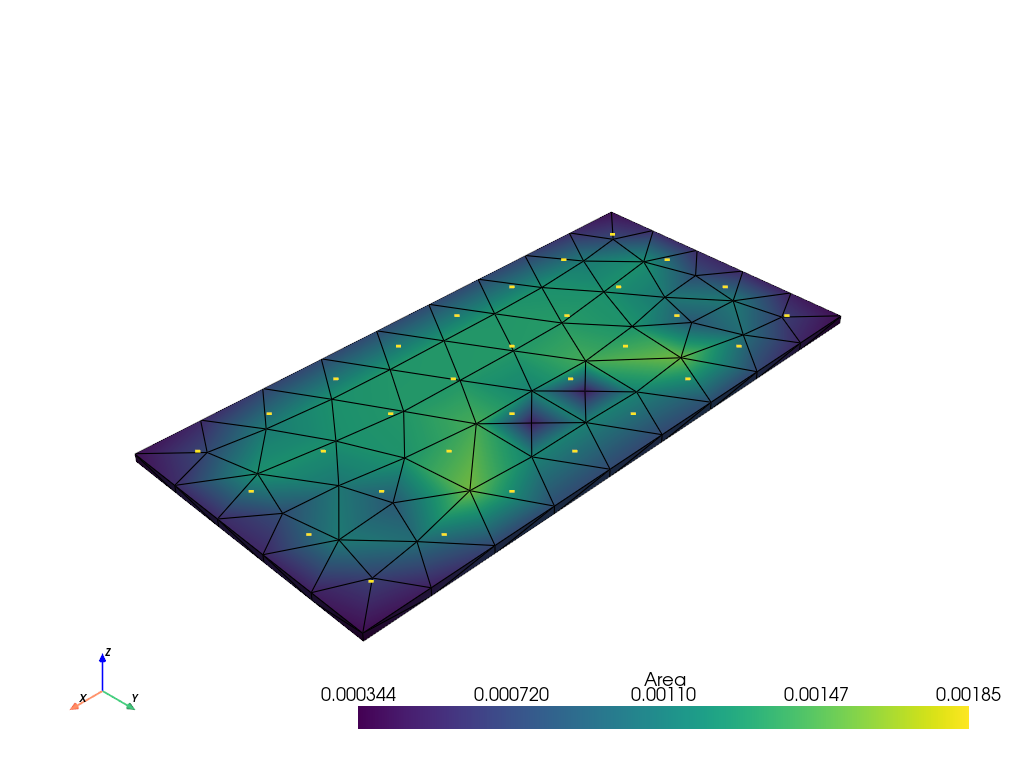
Visualisation of the Modelled Array
Once the antenna array has been generated for simulation, it can then be visualised within the model space, and a rendering exported.
pl = pv.Plotter()
pl.add_mesh(elements)
pl.add_mesh(pv.from_meshio(panel), show_edges=True)
pl.add_axes()
pl.show(screenshot="ArrayasSimulated.png")
Definition of the sample field and simulation
In order to make comparisons straightforward, the sample field positions are copied from the measured data while removing the actual field data itself. The excitation_function is called to allow the definition of electric field vectors for each antenna with the same polarization as produced by the patch antennas of the validation antenna array.
import lyceanem.models.frequency_domain as FD
from lyceanem.electromagnetics.emfunctions import excitation_function

desired_e_vector = np.array([1.0, 0.0, 0])
weights = excitation_function(
    elements,
    desired_e_vector,
    wavelength=wavelength,
    phase_shift="wavefront",
    steering_vector=np.array([0, 0, 1]),
)


sample_field = antennas[0].copy()
sample_field.point_data.clear()
sample_field.point_data["Normals"] = antennas[0].point_data["Normals"]

from lyceanem.base_classes import structures

blockers = structures(solids=[panel])
Ex, Ey, Ez = FD.calculate_scattering(
    aperture_coords=elements,
    sink_coords=sample_field,
    scatter_points=panel,
    antenna_solid=blockers,
    desired_E_axis=weights,
    wavelength=wavelength,
    scattering=0,
    project_vectors=False,
    beta=(2 * np.pi) / wavelength,
)
C:\Users\lycea\miniconda3\envs\CudaDevelopment\Lib\site-packages\lyceanem\electromagnetics\empropagation.py:3719: ComplexWarning: Casting complex values to real discards the imaginary part
  uvn_axes[2, :] = point_vector
C:\Users\lycea\miniconda3\envs\CudaDevelopment\Lib\site-packages\lyceanem\electromagnetics\empropagation.py:3731: ComplexWarning: Casting complex values to real discards the imaginary part
  uvn_axes[0, :] = np.cross(local_axes[0, :], point_vector) / np.linalg.norm(
C:\Users\lycea\miniconda3\envs\CudaDevelopment\Lib\site-packages\lyceanem\electromagnetics\empropagation.py:3758: ComplexWarning: Casting complex values to real discards the imaginary part
  uvn_axes[1, :] = np.cross(point_vector, uvn_axes[0, :]) / np.linalg.norm(
Processing of the Modelled results
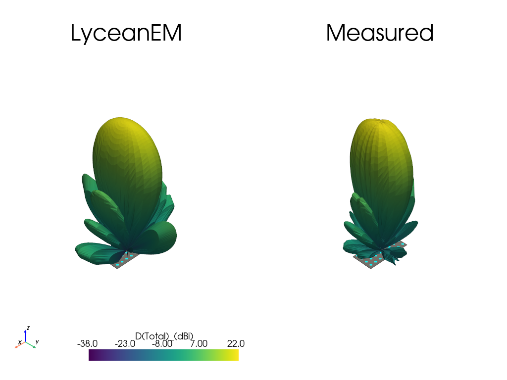
The function update_electric_fields is used to populate the sample field with the simulated farfield pattern of the antenna array with the calculated weights. A wide variety of different quantities can then be calculated to allow consistent analysis of the measured and simulated antenna patterns.
from lyceanem.electromagnetics.emfunctions import (
    update_electric_fields,
    PoyntingVector,
    Directivity,
    Exyz_to_EthetaEphi,
    field_magnitude_phase,
)
from lyceanem.electromagnetics.beamforming import create_display_mesh

measured_array_pattern = field_magnitude_phase(
    Directivity(PoyntingVector(Beamform(antennas, weights[:, 1])))
)
dynamic_range = 60
sample_field = field_magnitude_phase(
    Directivity(PoyntingVector(update_electric_fields(sample_field, Ex, Ey, Ez)))
)
display = create_display_mesh(
    sample_field, label="D(Total)", field_radius=1.0, dynamic_range=dynamic_range
)
display.point_data["D(Total)_(dBi)"] = 10 * np.log10(display.point_data["D(Total)"])
measured_display = create_display_mesh(
    measured_array_pattern,
    label="D(Total)",
    field_radius=1.0,
    dynamic_range=dynamic_range,
)
measured_display.point_data["D(Total)_(dBi)"] = 10 * np.log10(
    measured_display.point_data["D(Total)"]
)

print("Maximum Directivity ", np.max(display.point_data["D(Total)_(dBi)"]))
print(
    "Measured Maximum Directivity ",
    np.max(measured_display.point_data["D(Total)_(dBi)"]),
)

pl = pv.Plotter(shape=(1, 2), border=False)
pl.subplot(0, 0)
pl.add_mesh(elements, color="aqua")
pl.add_mesh(panel, color="grey")
pl.add_mesh(display, scalars="D(Total)_(dBi)", clim=[22 - dynamic_range, 22])
pl.add_axes()
pl.add_title("LyceanEM")
pl.subplot(0, 1)
pl.add_mesh(elements, color="aqua")
pl.add_mesh(panel, color="grey")
pl.add_mesh(measured_display, scalars="D(Total)_(dBi)", clim=[22 - dynamic_range, 22])
pl.add_title("Measured")
pl.link_views()
pl.view_isometric()
pl.show(screenshot="MeasurementtoSimulationComparison.png")


simulated = display.point_data["D(Total)"]
measured = measured_display.point_data["D(Total)"]
print(
    "Correlation {}".format(np.corrcoef(simulated, measured)[0, 1]),
    " between measurement and simulation",
)
C:\Users\lycea\miniconda3\envs\CudaDevelopment\Lib\site-packages\lyceanem\electromagnetics\emfunctions.py:539: RuntimeWarning: divide by zero encountered in log10
  field_data.point_data["Poynting_Vector_(Magnitude_(dBW/m2))"] = 10 * np.log10(
C:\Users\lycea\miniconda3\envs\CudaDevelopment\Lib\site-packages\lyceanem\electromagnetics\beamforming.py:1617: RuntimeWarning: divide by zero encountered in log10
  logdata = log_multiplier * np.log10(pattern_mesh.point_data[label])
C:\Users\lycea\PycharmProjects\LyceanEM-Python\docs\source\examples\08_array_validation.py:249: RuntimeWarning: divide by zero encountered in log10
  display.point_data["D(Total)_(dBi)"] = 10 * np.log10(display.point_data["D(Total)"])
Maximum Directivity  20.07648569434074
Measured Maximum Directivity  21.082011910586985
Correlation 0.9966437988952569  between measurement and simulation
Total running time of the script: (1 minutes 8.238 seconds)